Exploring Spelunker tools and features
Authors: Derod Deal (dealderod@ufl.edu), Néstor Espinoza (nespinoza@stsci.edu) | Last update: January 22, 2024
Program version: ver. 1.1.9
The JWST telescope carries four different instruments: NIRCam, NIRSpec, MIRI and FGS/NIRISS — the latter containing the Fine Guidance Sensor (FGS). FGS Spelunker is a package designed to conveniently analyze guidestar data. In this notebook, we cover the following main functions of this package.
-
Installation
Using
Spelunker
Spatial fitting guide stars
Periodograms
Getting started
To get started with FGS Spelunker, first call spelunker.load into a
variable while setting a given Program ID.
import spelunker
spk = spelunker.load(pid=1534)
Calling load without the pid parameter spelunker.load() will
initialize spelunker without downloading any of the files. This is
useful if you already have guidestar FITS available locally.
Downloading data
To load Spelunker with a given Program ID for JWST, simply call
spelunker.load with the Program ID pid as a parameter. This will
create a directory called spelunker_results, which is where the FITS
files from a selected Program ID and other data will be downloaded and
saved. You can define your own directory by using dir=.
The Program IDs that can be loaded are limited to programs without an exclusive access period or are available publicly (https://jwst-docs.stsci.edu/accessing-jwst-data/jwst-data-retrieval/data-access-policy#DataAccessPolicy-Exclusiveaccessperiod).
import spelunker
spk = spelunker.load(dir='/Users/ddeal/JWST-Treasure-Chest/', pid='1534')
Current working directory for spelunker: /Users/ddeal/JWST-Treasure-Chest/spelunker_outputs

Connecting with astroquery...
INFO: Found cached file ./mastDownload/JWST/jw01534002002_04101_00001_guider2/jw01534002002_gs-fg_2022338021919_cal.fits with expected size 10428480. [astroquery.query]
INFO: Found cached file ./mastDownload/JWST/jw01534001004_03101_00001_guider1/jw01534001004_gs-fg_2022340010755_cal.fits with expected size 8766720. [astroquery.query]
INFO: Found cached file ./mastDownload/JWST/jw01534002004_03101_00001_guider2/jw01534002004_gs-fg_2022338025056_cal.fits with expected size 8769600. [astroquery.query]
INFO: Found cached file ./mastDownload/JWST/jw01534001002_03101_00001_guider1/jw01534001002_gs-fg_2022340003651_cal.fits with expected size 8772480. [astroquery.query]
INFO: Found cached file ./mastDownload/JWST/jw01534002003_03101_00001_guider2/jw01534002003_gs-fg_2022338023521_cal.fits with expected size 8772480. [astroquery.query]
INFO: Found cached file ./mastDownload/JWST/jw01534001003_03101_00001_guider1/jw01534001003_gs-fg_2022340005224_cal.fits with expected size 8772480. [astroquery.query]
INFO: Found cached file ./mastDownload/JWST/jw01534002001_05101_00002_guider2/jw01534002001_gs-fg_2022338014704_cal.fits with expected size 10941120. [astroquery.query]
INFO: Found cached file ./mastDownload/JWST/jw01534002001_05101_00002_guider2/jw01534002001_gs-fg_2022338015941_cal.fits with expected size 7830720. [astroquery.query]
INFO: Found cached file ./mastDownload/JWST/jw01534001001_03101_00002_guider1/jw01534001001_gs-fg_2022340000825_cal.fits with expected size 9388800. [astroquery.query]
INFO: Found cached file ./mastDownload/JWST/jw01534001001_03101_00002_guider1/jw01534001001_gs-fg_2022340002102_cal.fits with expected size 7827840. [astroquery.query]
INFO: Found cached file ./mastDownload/JWST/jw01534004004_03101_00001_guider2/jw01534004004_gs-fg_2023123213436_cal.fits with expected size 8769600. [astroquery.query]
INFO: Found cached file ./mastDownload/JWST/jw01534004003_03101_00001_guider2/jw01534004003_gs-fg_2023123211905_cal.fits with expected size 8766720. [astroquery.query]
INFO: Found cached file ./mastDownload/JWST/jw01534004002_03101_00001_guider2/jw01534004002_gs-fg_2023123210335_cal.fits with expected size 8766720. [astroquery.query]
INFO: Found cached file ./mastDownload/JWST/jw01534004001_03101_00002_guider2/jw01534004001_gs-fg_2023123203053_cal.fits with expected size 12974400. [astroquery.query]
INFO: Found cached file ./mastDownload/JWST/jw01534004001_03101_00002_guider2/jw01534004001_gs-fg_2023123204330_cal.fits with expected size 7827840. [astroquery.query]
INFO: Found cached file ./mastDownload/JWST/jw01534003001_03101_00002_guider1/jw01534003001_gs-fg_2023125174543_cal.fits with expected size 9809280. [astroquery.query]
INFO: Found cached file ./mastDownload/JWST/jw01534003001_03101_00002_guider1/jw01534003001_gs-fg_2023125175812_cal.fits with expected size 7793280. [astroquery.query]
INFO: Found cached file ./mastDownload/JWST/jw01534003002_02101_00001_guider1/jw01534003002_gs-fg_2023125181351_cal.fits with expected size 8337600. [astroquery.query]
INFO: Found cached file ./mastDownload/JWST/jw01534003003_02101_00001_guider1/jw01534003003_gs-fg_2023125182911_cal.fits with expected size 8337600. [astroquery.query]
INFO: Found cached file ./mastDownload/JWST/jw01534003004_02101_00001_guider1/jw01534003004_gs-fg_2023125185519_cal.fits with expected size 8337600. [astroquery.query]
To download the data after initialization, use spk.download() with
given proposal id with the optional parameters observation number
obs_num and visit number visit. You can also set the calibration
level calib_level. This information are required to use
astroquery.mast to search and download the necessary files. The
download function will download the selected files in the given
directory and create a 2D array of the guidestar data as well as an
array of time and a flux timeseries. The same parameters work with
spelunker.load.
spk2 = spelunker.load(pid=1534, obs_num='2', visit='1', calib_level=2)
spk2.download(1534, obs_num='2', visit='2', calib_level=2) # This overwrites the object data in spk2 with data from the input parameters
Current working directory for spelunker: /Users/ddeal/JWST-Treasure-Chest/spelunker_outputs

Connecting with astroquery...
2023-08-02 21:11:34,101 - stpipe - INFO - Found cached file ./mastDownload/JWST/jw01534002001_05101_00002_guider2/jw01534002001_gs-fg_2022338014704_cal.fits with expected size 10941120.
2023-08-02 21:11:34,195 - stpipe - INFO - Found cached file ./mastDownload/JWST/jw01534002001_05101_00002_guider2/jw01534002001_gs-fg_2022338015941_cal.fits with expected size 7830720.
INFO: Found cached file ./mastDownload/JWST/jw01534002001_05101_00002_guider2/jw01534002001_gs-fg_2022338014704_cal.fits with expected size 10941120. [astroquery.query]
INFO: Found cached file ./mastDownload/JWST/jw01534002001_05101_00002_guider2/jw01534002001_gs-fg_2022338015941_cal.fits with expected size 7830720. [astroquery.query]
Connecting with astroquery...
2023-08-02 21:11:41,186 - stpipe - INFO - Found cached file ./mastDownload/JWST/jw01534002002_04101_00001_guider2/jw01534002002_gs-fg_2022338021919_cal.fits with expected size 10428480.
INFO: Found cached file ./mastDownload/JWST/jw01534002002_04101_00001_guider2/jw01534002002_gs-fg_2022338021919_cal.fits with expected size 10428480. [astroquery.query]
After we downloaded our data, we can access preprocessed spatial, time,
and flux arrays for all FITS files images under the specified Program
ID. Use the attributes spk.fg_array, spk.fg_time, and
spk.fg_flux to access the arrays.
spk2.fg_array.shape, spk2.fg_time.shape, spk2.fg_flux.shape
((10240, 8, 8), (10240,), (10240,))
Previously downloaded FITS files in a given directory will not be
re-downloaded. If there are multiple files downloaded for the given
parameter, spk.download will automatically stitch the data from the
files into an array based on the date and time for each file, along with
the time and flux arrays.
FGS Spelunker can also handle guidestar FITS already stored locally by using:
spk2 = spelunker.load()
spk2.readfile(pid=1534)
Any files under the initialized directory and specified Program ID, observation number, and visit number will be loaded into spk2.
spelunker.load.readfilenow has access to the same attributes asspelunker.load.download. So, usingspk.object_propertiesandspk.fg_tablewill work.
Spatial fitting guide stars
After downloading the data, we can perform spatial fitting gaussians to
each frame in a guidestar timeseries. This uses parallel processing
through ray to speed up the process. We can also perform quick fits
to speed through a given timeseries, though this method is a lot less
accurate in the fitting.
Gaussian fitting
The downloaded data comes as a spatial timeseries of a selected
guidestar. To measure the centriods and PSF width of each frame, we need
to apply fitting. We will use Gaussian spatial fitting to measure x and
y pixel coordinates, x and y standard deviations, theta, and the
offset. To perform spatial gaussian fitting, use gauss2d_fit with guidestar arrays (the
timeseries needs to be in an 8 by 8 array, which should be the same for
all guidestar fine guidence products).
spk.gauss2d_fit() # ncpus sets the number of cpu cores your computer has. Defaults to 4 cores.
# We are going to limit the amount of frames that we input into gauss2d_fit and other methods
# since the gauss2d_fit can take a few houts for very large arrays.
spk.fg_array = spk.fg_array[0:10000]
spk.fg_flux = spk.fg_flux[0:10000]
spk.fg_time = spk.fg_time[0:10000]
table_gauss_fit = spk.gauss2d_fit(ncpus=6)
2023-08-02 21:12:50,384 INFO worker.py:1636 -- Started a local Ray instance.
The gauss2d_fit function outputs an astropy table, which can bee
accessed with the spk.gaussfit_results attribute. If gauss2d_fit
fails to fit a frame, it will return nan for that frame.
spk.gaussfit_results
| amplitude | x_mean | y_mean | x_stddev | y_stddev | theta | offset |
|---|---|---|---|---|---|---|
| float64 | float64 | float64 | float64 | float64 | float64 | float64 |
| 280706.15465765796 | 3.1774294356249997 | 2.7465302838135206 | 0.6350976070387301 | 0.614009020575321 | -1.9103595130650228 | 3023.106318279726 |
| 280706.15465765796 | 3.1774294356249997 | 2.7465302838135206 | 0.6350976070387301 | 0.614009020575321 | -1.9103595130650228 | 3023.106318279726 |
| 280963.5540504813 | 3.177604462333186 | 2.7483597462452547 | 0.6306454543965104 | 0.6193386849707871 | -2.057972902746876 | 3149.3240730860866 |
| 280963.5540504813 | 3.177604462333186 | 2.7483597462452547 | 0.6306454543965104 | 0.6193386849707871 | -2.057972902746876 | 3149.3240730860866 |
| 282706.5250312361 | 3.1764861837068716 | 2.749817871515913 | 0.6334273199822001 | 0.6145497343103167 | -1.9504191092501943 | 3053.0948632606123 |
| 282706.5250312361 | 3.1764861837068716 | 2.749817871515913 | 0.6334273199822001 | 0.6145497343103167 | -1.9504191092501943 | 3053.0948632606123 |
| 277126.33630266984 | 3.1748827601728564 | 2.7477495874396674 | 0.6189797899040209 | 0.6340116557887706 | -3.48449959258196 | 3105.682301707251 |
| 277126.33630266984 | 3.1748827601728564 | 2.7477495874396674 | 0.6189797899040209 | 0.6340116557887706 | -3.48449959258196 | 3105.682301707251 |
| 280742.3344982786 | 3.1719030737999923 | 2.756636337651271 | 0.6154040193075433 | 0.6363143600933248 | -3.570644823307217 | 3017.796074602062 |
| 280742.3344982786 | 3.1719030737999923 | 2.756636337651271 | 0.6154040193075433 | 0.6363143600933248 | -3.570644823307217 | 3017.796074602062 |
| ... | ... | ... | ... | ... | ... | ... |
| 288936.6587997144 | 3.1514848995974614 | 2.816421337922728 | 0.6078414078127158 | 0.6255153338398373 | -0.724102219944298 | 3159.747623016102 |
| 288936.6587997144 | 3.1514848995974614 | 2.816421337922728 | 0.6078414078127158 | 0.6255153338398373 | -0.724102219944298 | 3159.747623016102 |
| 287608.5204882826 | 3.148081209519121 | 2.8097574913336154 | 0.6092268378675755 | 0.6288855374510539 | -0.6364418904422164 | 3098.4078599410695 |
| 287608.5204882826 | 3.148081209519121 | 2.8097574913336154 | 0.6092268378675755 | 0.6288855374510539 | -0.6364418904422164 | 3098.4078599410695 |
| 286304.0727626729 | 3.1471623118694176 | 2.8102083208968813 | 0.6085355521172578 | 0.6298236704220975 | -0.5591615297330863 | 3183.299010073181 |
| 286304.0727626729 | 3.1471623118694176 | 2.8102083208968813 | 0.6085355521172578 | 0.6298236704220975 | -0.5591615297330863 | 3183.299010073181 |
| 284871.6486689821 | 3.1499465078006614 | 2.8072167275653706 | 0.6111915236092285 | 0.6277931861719188 | -0.7047253049826113 | 3261.2487765038327 |
| 284871.6486689821 | 3.1499465078006614 | 2.8072167275653706 | 0.6111915236092285 | 0.6277931861719188 | -0.7047253049826113 | 3261.2487765038327 |
| 288107.09702730743 | 3.14940434535617 | 2.807916552216667 | 0.6081505348286508 | 0.6295003348022744 | -0.6030650650578055 | 3197.4098077599647 |
| 288107.09702730743 | 3.14940434535617 | 2.807916552216667 | 0.6081505348286508 | 0.6295003348022744 | -0.6030650650578055 | 3197.4098077599647 |
Quick fitting
There are some situations where you need to quickly obtain rough
statistics of changes in guidestar products overtime. Quick fitting fits
the x and y pixel locations and standard deviations as an astropy table
using centroid and variance calculations. To perform quick fitting, run
quick_fit with an appropriate array.
table_quick_fit = spk.quick_fit()
spk.quickfit_results
| amplitude | x_mean | y_mean | x_stddev | y_stddev | theta | offset |
|---|---|---|---|---|---|---|
| float32 | float64 | float64 | float64 | float64 | int64 | int64 |
| 254451.56 | 3.240314850861845 | 2.8033942297495758 | 1.74462175414244 | 1.8158228238188503 | 0 | 0 |
| 254451.56 | 3.240314850861845 | 2.8033942297495758 | 1.74462175414244 | 1.8158228238188503 | 0 | 0 |
| 255055.25 | 3.3206004778017384 | 2.8434574303565463 | 1.8543257785557397 | 1.8293394846671764 | 0 | 0 |
| 255055.25 | 3.3206004778017384 | 2.8434574303565463 | 1.8543257785557397 | 1.8293394846671764 | 0 | 0 |
| 256947.42 | 3.3505845162736376 | 2.925690858450849 | 1.8077292667969422 | 1.8943471255043283 | 0 | 0 |
| 256947.42 | 3.3505845162736376 | 2.925690858450849 | 1.8077292667969422 | 1.8943471255043283 | 0 | 0 |
| 251888.12 | 3.3039389301600726 | 2.886233231270987 | 1.854677926018813 | 1.8433178905598915 | 0 | 0 |
| 251888.12 | 3.3039389301600726 | 2.886233231270987 | 1.854677926018813 | 1.8433178905598915 | 0 | 0 |
| 257109.62 | 3.2835164773971806 | 2.774318082677534 | 1.837107063709473 | 1.7647732623026264 | 0 | 0 |
| 257109.62 | 3.2835164773971806 | 2.774318082677534 | 1.837107063709473 | 1.7647732623026264 | 0 | 0 |
| ... | ... | ... | ... | ... | ... | ... |
| 273886.84 | 3.307248070570433 | 2.9459581137888096 | 1.8638542966133642 | 1.8248573282234368 | 0 | 0 |
| 273886.84 | 3.307248070570433 | 2.9459581137888096 | 1.8638542966133642 | 1.8248573282234368 | 0 | 0 |
| 272548.8 | 3.303274024993382 | 2.888558147490168 | 1.8282836367085207 | 1.7580760556837993 | 0 | 0 |
| 272548.8 | 3.303274024993382 | 2.888558147490168 | 1.8282836367085207 | 1.7580760556837993 | 0 | 0 |
| 271490.1 | 3.228820447972362 | 3.055912219282716 | 1.8189049613644188 | 1.8755066513378191 | 0 | 0 |
| 271490.1 | 3.228820447972362 | 3.055912219282716 | 1.8189049613644188 | 1.8755066513378191 | 0 | 0 |
| 269606.9 | 3.328221486759065 | 2.963716959723631 | 1.8706223659386954 | 1.8586654374692335 | 0 | 0 |
| 269606.9 | 3.328221486759065 | 2.963716959723631 | 1.8706223659386954 | 1.8586654374692335 | 0 | 0 |
| 272629.9 | 3.304655431094987 | 2.9615702404863526 | 1.873261996709939 | 1.9288479581727678 | 0 | 0 |
| 272629.9 | 3.304655431094987 | 2.9615702404863526 | 1.873261996709939 | 1.9288479581727678 | 0 | 0 |
Plotting parameters
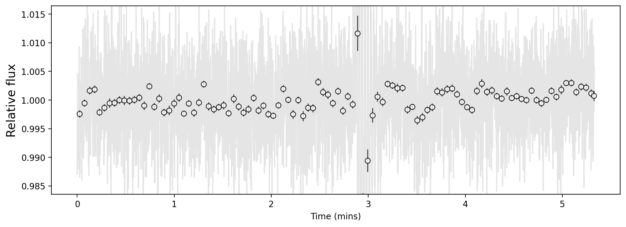
We can plot a timeseries of a given parameter or flux from guidestars.
The method timeseries_binned_plot will generate a matplotlib axes
object of a given timeseries.
import matplotlib.pyplot as plt
fig, ax = plt.subplots(figsize = (12,4), dpi=200)

ax = spk.timeseries_binned_plot()
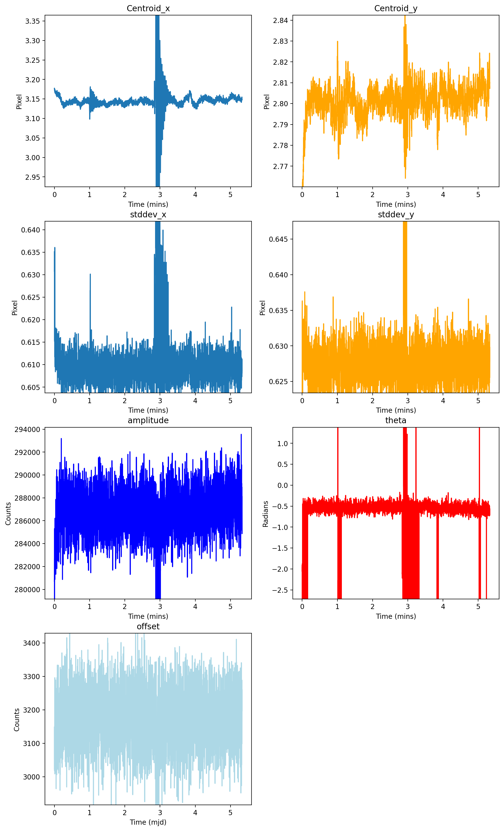
Within guidestar data, changes in the PSF can impact the observed flux of the star. Certain events might see changes in all fitted parameters. In this case, subplots of each parameter will provide more information to the user about the event, giving them the change of guidestar position, brightness, and FWHM overtime.
ax = spk.timeseries_list_plot()
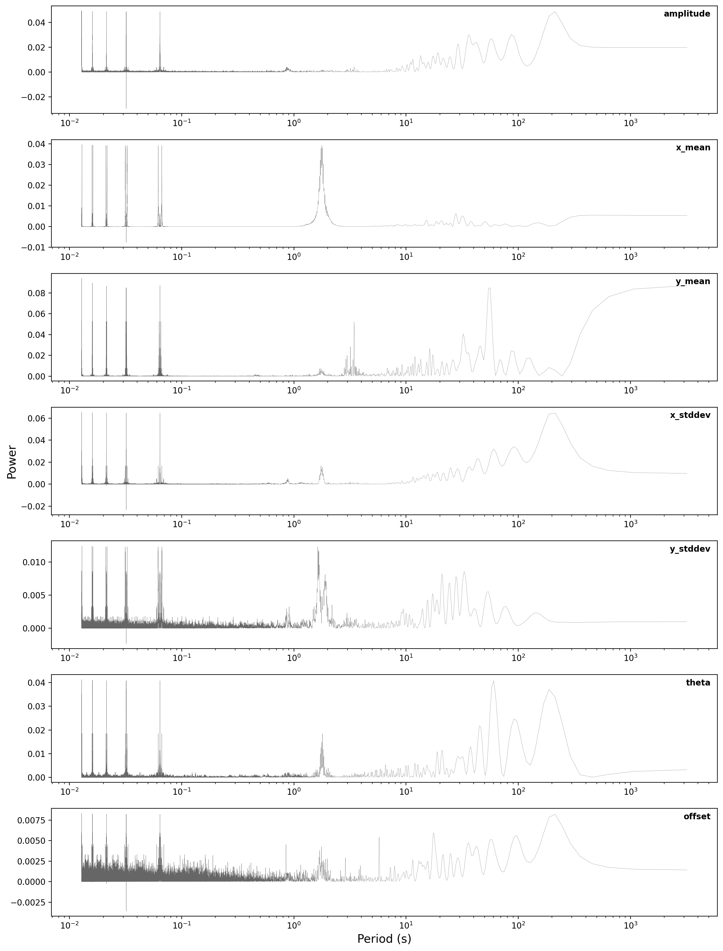
Periodograms
FGS Spelunker comes with various tools to visualize and explore guidestar data. Periodograms are useful for guidestar products to detect periodicities not only within flux timeseries, but also within centroids, FWHM, theta, and offset. From a selected fitting method, we can use the table output to apply Lomb-Scargle periodograms to our parameters.
periodogram
To obtain the power and frequencies of Lomb-Scargle periodograms for
each fitted parameter, use periodogram. The periodograms for each
given parameter from a fit can be conveniently plotted in a single
figure with the same method.
ax = spk.periodogram()
To get the frequency and power for each fitted parameter, use
spk.pgram_{parameter}.
Available parameters:
spk.pgram_amplitudespk.pgram_x_meanspk.pgram_y_meanspk.pgram_x_stddevspk.pgram_y_stddevspk.pgram_thetaspk.pgram_offset
freq = spk.pgram_x_mean[0] # periodogram frequency
power = spk.pgram_x_mean[1] # periodogram power

freq[0], power[0]
(0.0003127661546504965, 0.005397779092056495)
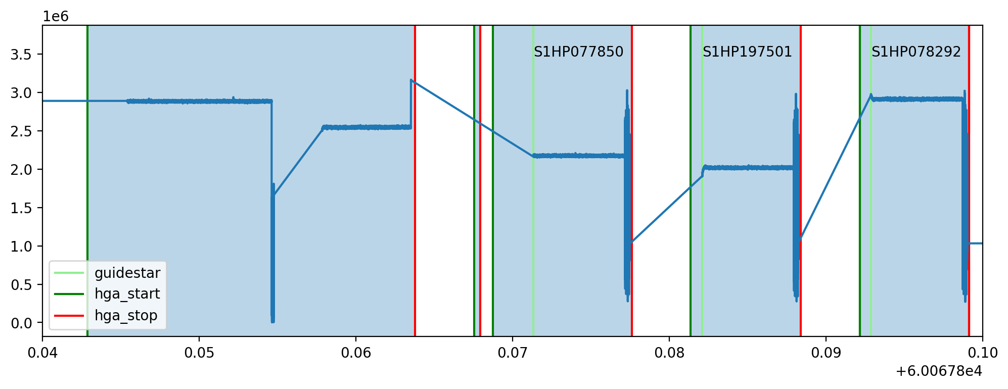
Mnemonics
When observing the timeseries of the guidestar, there might be technical
events from the JWST that causes changes in obtained data. For example,
high gain antenna or filter changes in NIRCAM can cause noticeable
changes in flux or other guidestar properties. We can overlay these
events onto fitted parameters using mnemonics and
mnemonics_plot. You will need a MAST API token to use mnemonics,
as well as the jwstuser package:
(MAST API TOKEN) - https://github.com/spacetelescope/jwstuser/tree/main (jwstuser)
Current supported mnemonics:
SA_ZHGAUPST (high-gain antenna),
INIS_FWMTRCURR (NIRISS Filter Wheel Motor Current).
There are thousands of different mnemonics to explore on https://mast.stsci.edu/viz/api/v0.1/info/mnemonics. Use spk.mnemonics to try the mnemonics you are interested in comparing with any JWST data, not just guidestars from the FGS.
spk2 = spelunker.load('/Users/ddeal/JWST-Treasure-Chest/', pid=1534)
spk2.mast_api_token = 'enter_mast_token_id_here' # input mast_api token here!

fig, ax = plt.subplots(figsize=(12,4),dpi=200)

ax = spk2.mnemonics_local('GUIDESTAR') # plots when the JWST tracks onto a new guidestars as a vertical line
ax = spk2.mnemonics('SA_ZHGAUPST', 60067.84, 60067.9) # plots the start and end of high gain antenna movement

ax.plot(spk2.fg_time, spk2.fg_flux)
plt.legend(loc=3)

plt.xlim(60067.84, 60067.9)
If you do have a MAST API token, you will have access to any program under that token.
If you do not have access to a MAST API token, you can only download and use publicly available Program IDs. However, with the readfile function, you can use fine guidance files you already have downloaded locally, and with the current version, with no drawbacks.
Animations
Spatial data of guidestar imaging can bring essential information about
how the point spread function changes overtime. Animations of the
spatial timeseries are convenient and helpful methods to analyze
guidestar data. To get a side by side comparison of the evolution of a
spatial timeseries and a parameter, use
flux_spatial_timelapse_animation.
You may have to install
ffmpegon your computer to getmp4formats.
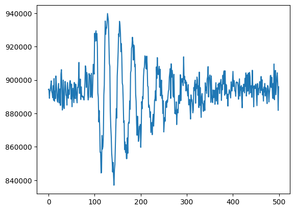
plt.plot(spk2.fg_flux[2600:3100])
[<matplotlib.lines.Line2D at 0x1c16b7550>]
spk2.flux_spatial_timelapse_animation(start=2600,stop=3100,) # to save an animation with a filename, use *filename=*. Defaults to movie.gif
2023-08-02 21:19:50,803 INFO worker.py:1636 -- Started a local Ray instance.

Getting tables
After downloading a selected proposal id with download, we can
easily output metadata about each downloaded file, including extracted
data from the filename including visit_group,
parallel_sequence_id, and exposure_number. The guide star used
in each file is also included, as well as filter magnitudes and other
stellar properties.
spk.fg_table # We can simply call this attribute after using spk.download() to obtain our table!
We can obtain a neat DataFrame of each tracked guidestar, which gives us information such as the intergation start times and galactic coordinates.
spk.object_properties
| guidestar_catalog_id | gaiadr1ID | gaiadr2ID | int_start | int_stop | ra | dec | Jmag | Hmag | |
|---|---|---|---|---|---|---|---|---|---|
| 0 | S1HP079555 | 4658077781377287680 | 4658077781376437888 | 59917.066396 | 59917.074354 | 80.837584 | -69.541124 | 13.659 | 12.898 |
| 1 | S1HP080554 | 4658077991763987712 | 4658077991799023616 | 59917.089163 | 59917.096759 | 80.806837 | -69.530972 | 15.001 | 14.282 |
| 2 | S1HP078573 | 4657983910572904320 | 4657983910572904320 | 59917.112547 | 59917.118705 | 80.807043 | -69.553474 | 13.839 | 13.078 |
| 3 | S1HP079590 | 4657986831103727872 | 4657986835382982016 | 59918.999015 | 59919.005848 | 80.510790 | -69.545479 | 15.410 | 14.839 |
| 4 | S1HP079769 | 4657986831078120832 | 4657986835433225728 | 59919.019436 | 59919.025598 | 80.518235 | -69.543415 | 15.231 | 14.341 |
| 5 | S1HP078292 | 4657986796681532672 | 4657986801073794432 | 59919.041018 | 59919.047165 | 80.519564 | -69.558464 | 12.804 | 11.883 |
| 6 | S1HP077850 | 4657986762384054144 | 4657986766713867264 | 60067.871344 | 60067.877490 | 80.573531 | -69.562862 | 12.957 | 12.227 |
| 7 | S1HP197501 | 4657986865463528832 | 4657986869793061376 | 60067.882117 | 60067.888264 | 80.571447 | -69.551750 | 13.063 | 12.168 |
| 8 | S1HP773376 | 4658078124973829632 | 60069.733171 | 60069.740086 | 80.794522 | -69.504084 | 13.426 | 12.654 | |
| 9 | S1HP081366 | 4658078056254368128 | 4658078056254368128 | 60069.753592 | 60069.759620 | 80.758291 | -69.524143 | 12.765 | 11.899 |
| 10 | S1HP082164 | 4658077953064455552 | 4658077957439332608 | 60069.764246 | 60069.770278 | 80.865554 | -69.514107 | 12.753 | 11.871 |